How To Find Average Acceleration On A Velocity Time Graph

3 Move Forth a Direct Line

3.3 Boilerplate and Instantaneous Acceleration

Learning Objectives

By the stop of this section, you will exist able to:

• Summate the average acceleration between two points in time.
• Calculate the instantaneous acceleration given the functional form of velocity.
• Explain the vector nature of instantaneous acceleration and velocity.
• Explain the difference between average dispatch and instantaneous acceleration.
• Find instantaneous acceleration at a specified time on a graph of velocity versus fourth dimension.

The importance of understanding acceleration spans our 24-hour interval-to-twenty-four hours experience, likewise every bit the vast reaches of outer infinite and the tiny world of subatomic physics. In everyday conversation, to accelerate ways to speed up; applying the restriction pedal causes a vehicle to dull down. We are familiar with the acceleration of our auto, for case. The greater the acceleration, the greater the alter in velocity over a given time. Acceleration is widely seen in experimental physics. In linear particle accelerator experiments, for example, subatomic particles are accelerated to very high velocities in collision experiments, which tell us information about the structure of the subatomic world also as the origin of the universe. In infinite, cosmic rays are subatomic particles that have been accelerated to very loftier energies in supernovas (exploding massive stars) and active galactic nuclei. It is important to understand the processes that accelerate cosmic rays because these rays contain highly penetrating radiation that tin damage electronics flown on spacecraft, for instance.

Average Acceleration

The formal definition of acceleration is consistent with these notions just described, but is more than inclusive.

Average Dispatch

Average dispatch is the charge per unit at which velocity changes:

[latex]\overset{\text{–}}{a}=\frac{\Delta v}{\Delta t}=\frac{{five}_{\text{f}}-{5}_{0}}{{t}_{\text{f}}-{t}_{0}},[/latex]

where [latex]\overset{\text{−}}{a}[/latex] is average dispatch, v is velocity, and t is time. (The bar over the a ways average acceleration.)

Because acceleration is velocity in meters divided by time in seconds, the SI units for dispatch are frequently abbreviated m/s²—that is, meters per second squared or meters per second per second. This literally means past how many meters per 2d the velocity changes every second. Call back that velocity is a vector—information technology has both magnitude and direction—which ways that a change in velocity can be a change in magnitude (or speed), merely information technology tin can also be a change in management. For case, if a runner traveling at 10 km/h due east slows to a finish, reverses direction, continues her run at 10 km/h due west, her velocity has changed as a issue of the change in direction, although the magnitude of the velocity is the same in both directions. Thus, acceleration occurs when velocity changes in magnitude (an increase or decrease in speed) or in direction, or both.

Acceleration as a Vector

Acceleration is a vector in the same direction as the modify in velocity, [latex]\Delta v[/latex]. Since velocity is a vector, it can alter in magnitude or in direction, or both. Acceleration is, therefore, a change in speed or management, or both.

Keep in listen that although acceleration is in the direction of the modify in velocity, it is not always in the direction of movement. When an object slows down, its acceleration is opposite to the direction of its motility. Although this is commonly referred to every bit deceleration Figure, we say the train is accelerating in a management opposite to its direction of move.

Figure 3.10 A subway train in Sao Paulo, Brazil, decelerates as it comes into a station. It is accelerating in a management opposite to its direction of motility. (credit: Yusuke Kawasaki)

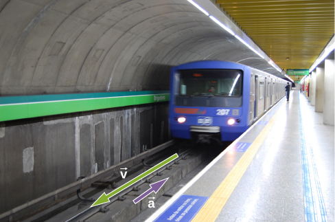
The term deceleration tin cause confusion in our assay considering it is not a vector and it does not indicate to a specific management with respect to a coordinate organisation, and then we do not use information technology. Acceleration is a vector, so we must cull the appropriate sign for information technology in our called coordinate system. In the instance of the railroad train in Figure, acceleration is in the negative direction in the chosen coordinate system, and so nosotros say the train is undergoing negative acceleration.

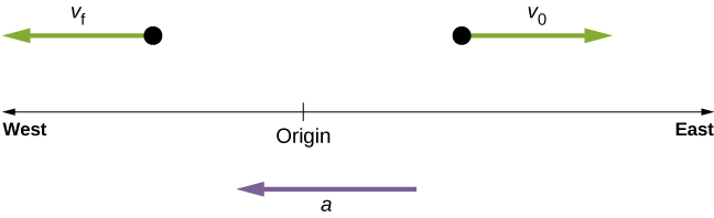
If an object in motion has a velocity in the positive management with respect to a chosen origin and it acquires a constant negative acceleration, the object somewhen comes to a residual and reverses direction. If we wait long enough, the object passes through the origin going in the contrary direction. This is illustrated in Figure.

Figure three.xi An object in motion with a velocity vector toward the east nether negative acceleration comes to a rest and reverses direction. It passes the origin going in the opposite management subsequently a long enough fourth dimension.

Example

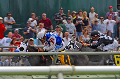
Calculating Average Acceleration: A Racehorse Leaves the Gate

A racehorse coming out of the gate accelerates from remainder to a velocity of 15.0 one thousand/s due west in one.fourscore s. What is its boilerplate acceleration?

Figure 3.12 Racehorses accelerating out of the gate. (credit: Jon Sullivan)

Strategy

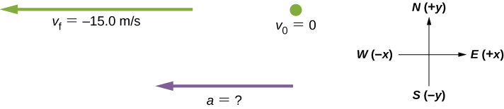
Starting time we draw a sketch and assign a coordinate system to the problem Figure. This is a simple problem, merely it always helps to visualize it. Observe that nosotros assign eastward equally positive and west as negative. Thus, in this case, we accept negative velocity.

Figure 3.13 Identify the coordinate arrangement, the given data, and what you desire to decide.

We can solve this problem by identifying [latex]\Delta v\,\text{and}\,\Delta t[/latex] from the given data, and so computing the average acceleration directly from the equation [latex]\overset{\text{–}}{a}=\frac{\Delta five}{\Delta t}=\frac{{five}_{\text{f}}-{five}_{0}}{{t}_{\text{f}}-{t}_{0}}[/latex].

Solution

First, identify the knowns: [latex]{v}_{0}=0,{5}_{\text{f}}=-15.0\,\text{m/s}[/latex] (the negative sign indicates direction toward the due west), Δt = one.eighty s.

Second, find the change in velocity. Since the horse is going from zero to –xv.0 m/south, its modify in velocity equals its final velocity:

[latex]\Delta 5={v}_{\text{f}}-{v}_{0}={v}_{\text{f}}=-fifteen.0\,\text{g/s}.[/latex]

Last, substitute the known values ([latex]\Delta v\,\text{and}\,\Delta t[/latex]) and solve for the unknown [latex]\overset{\text{–}}{a}[/latex]:

[latex]\overset{\text{–}}{a}=\frac{\Delta v}{\Delta t}=\frac{-15.0\,\text{m/s}}{1.fourscore\,\text{s}}=-8.33{\text{1000/due south}}^{2}.[/latex]

Significance

The negative sign for acceleration indicates that acceleration is toward the w. An acceleration of 8.33 grand/s² due west means the horse increases its velocity past 8.33 k/s due due west each second; that is, viii.33 meters per 2d per 2nd, which nosotros write equally 8.33 grand/sⁱⁱ. This is truly an boilerplate acceleration, because the ride is non shine. We see later that an dispatch of this magnitude would require the passenger to hang on with a forcefulness nearly equal to his weight.

Check Your Understanding

Protons in a linear accelerator are accelerated from rest to [latex]ii.0\times {10}^{seven}\,\text{m/southward}[/latex] in 10^–four s. What is the boilerplate acceleration of the protons?

Show Solution

Inserting the knowns, nosotros have

[latex]\overset{\text{–}}{a}=\frac{\Delta v}{\Delta t}=\frac{2.0\times {10}^{vii}\,\text{m/s}-0}{{10}^{-four}\,\text{s}-0}=2.0\times {10}^{11}{\text{m/southward}}^{2}.[/latex]

Instantaneous Acceleration

Instantaneous acceleration a, or acceleration at a specific instant in time, is obtained using the same process discussed for instantaneous velocity. That is, nosotros calculate the average velocity between two points in time separated by [latex]\Delta t[/latex] and let [latex]\Delta t[/latex] approach nix. The result is the derivative of the velocity office five(t), which is instantaneous dispatch and is expressed mathematically as

[latex]a(t)=\frac{d}{dt}v(t).[/latex]

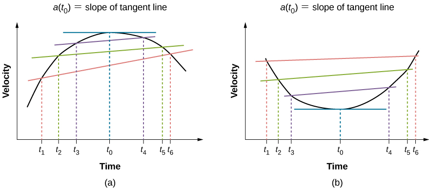
Thus, similar to velocity beingness the derivative of the position function, instantaneous acceleration is the derivative of the velocity role. We tin can show this graphically in the same manner every bit instantaneous velocity. In Figure, instantaneous dispatch at fourth dimension t ₀ is the gradient of the tangent line to the velocity-versus-time graph at time t ₀. Nosotros see that average acceleration [latex]\overset{\text{–}}{a}=\frac{\Delta 5}{\Delta t}[/latex] approaches instantaneous acceleration as [latex]\Delta t[/latex] approaches zero. Also in part (a) of the figure, nosotros see that velocity has a maximum when its slope is zero. This time corresponds to the zero of the acceleration function. In part (b), instantaneous acceleration at the minimum velocity is shown, which is also nil, since the slope of the curve is zero there, too. Thus, for a given velocity office, the zeros of the dispatch function give either the minimum or the maximum velocity.

Figure iii.14 In a graph of velocity versus fourth dimension, instantaneous acceleration is the slope of the tangent line. (a) Shown is average dispatch [latex]\overset{\text{–}}{a}=\frac{\Delta five}{\Delta t}=\frac{{5}_{\text{f}}-{v}_{i}}{{t}_{\text{f}}-{t}_{i}}[/latex] between times [latex]\Delta t={t}_{6}-{t}_{one},\Delta t={t}_{v}-{t}_{two}[/latex], and [latex]\Delta t={t}_{4}-{t}_{3}[/latex]. When [latex]\Delta t\to 0[/latex], the boilerplate dispatch approaches instantaneous acceleration at fourth dimension t0. In view (a), instantaneous acceleration is shown for the signal on the velocity curve at maximum velocity. At this betoken, instantaneous dispatch is the slope of the tangent line, which is zip. At whatever other time, the gradient of the tangent line—and thus instantaneous acceleration—would not be zilch. (b) Aforementioned equally (a) but shown for instantaneous acceleration at minimum velocity.

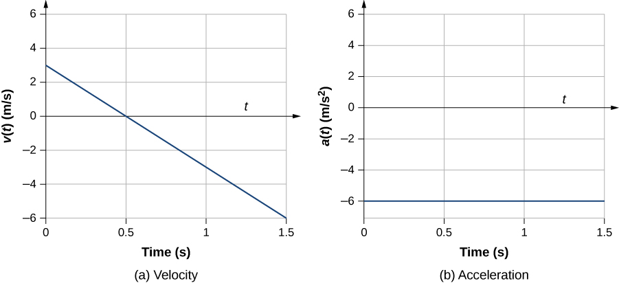
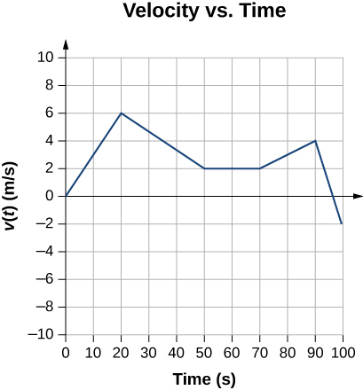
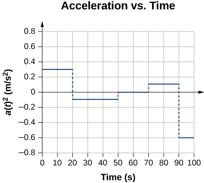
To illustrate this concept, let's look at 2 examples. Beginning, a simple instance is shown using Figure(b), the velocity-versus-time graph of Effigy, to detect acceleration graphically. This graph is depicted in Figure(a), which is a straight line. The respective graph of acceleration versus time is found from the gradient of velocity and is shown in Figure(b). In this example, the velocity role is a directly line with a constant slope, thus acceleration is a constant. In the adjacent example, the velocity function has a more complicated functional dependence on fourth dimension.

Figure three.15 (a, b) The velocity-versus-time graph is linear and has a negative constant slope (a) that is equal to acceleration, shown in (b).

If we know the functional grade of velocity, 5(t), we tin summate instantaneous acceleration a(t) at any time point in the motility using Figure.

Example

Calculating Instantaneous Acceleration

A particle is in motion and is accelerating. The functional form of the velocity is [latex]5(t)=20t-v{t}^{2}\,\text{k/s}[/latex].

1. Find the functional form of the dispatch.
2. Find the instantaneous velocity at t = i, 2, iii, and 5 s.
3. Find the instantaneous dispatch at t = 1, 2, three, and 5 due south.
4. Interpret the results of (c) in terms of the directions of the dispatch and velocity vectors.

Strategy

We observe the functional form of dispatch by taking the derivative of the velocity function. Then, we calculate the values of instantaneous velocity and dispatch from the given functions for each. For part (d), nosotros need to compare the directions of velocity and acceleration at each time.

Solution

1. [latex]a(t)=\frac{dv(t)}{dt}=20-10t\,{\text{m/s}}^{2}[/latex]
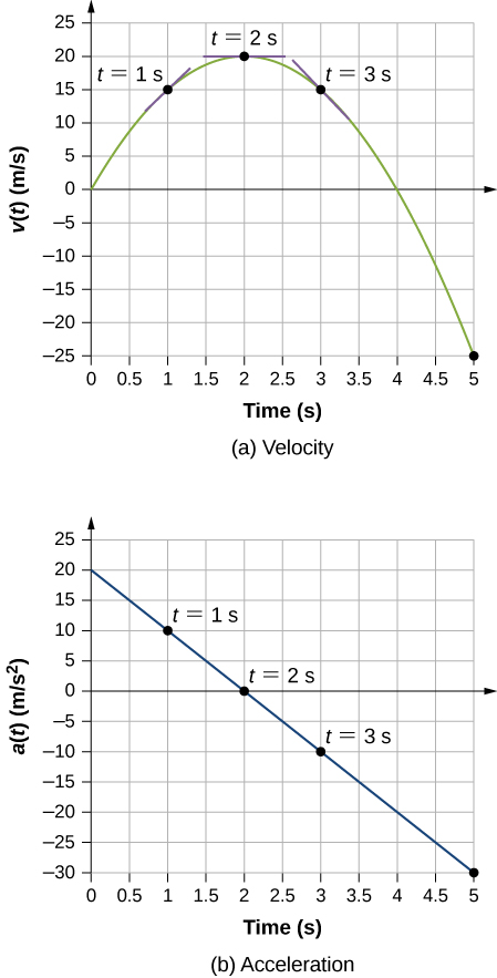
2. [latex]5(one\,\text{south})=15\,\text{chiliad/s}[/latex], [latex]v(ii\,\text{due south})=20\,\text{m/due south}[/latex], [latex]five(3\,\text{s})=fifteen\,\text{g/s}[/latex], [latex]5(v\,\text{due south})=-25\,\text{m/s}[/latex]
3. [latex]a(one\,\text{s})=x{\,\text{k/s}}^{ii}[/latex], [latex]a(2\,\text{s})=0{\,\text{k/s}}^{two}[/latex], [latex]a(three\,\text{due south})=-x{\,\text{m/s}}^{2}[/latex], [latex]a(5\,\text{s})=-30{\,\text{m/s}}^{2}[/latex]
4. At t = 1 southward, velocity [latex]v(1\,\text{s)}=15\,\text{m/s}[/latex] is positive and dispatch is positive, then both velocity and acceleration are in the same direction. The particle is moving faster.

At t = ii southward, velocity has increased to[latex]v(2\,\text{s)}=20\,\text{one thousand/s}[/latex], where it is maximum, which corresponds to the time when the acceleration is zero. We meet that the maximum velocity occurs when the gradient of the velocity function is zero, which is just the zero of the acceleration part.

At t = three s, velocity is [latex]5(three\,\text{s)}=xv\,\text{m/south}[/latex] and acceleration is negative. The particle has reduced its velocity and the dispatch vector is negative. The particle is slowing downwards.

At t = 5 due south, velocity is [latex]v(v\,\text{s)}=-25\,\text{m/southward}[/latex] and acceleration is increasingly negative. Between the times t = 3 s and t = 5 s the particle has decreased its velocity to zippo and then become negative, thus reversing its management. The particle is at present speeding up once again, but in the opposite direction.

We can see these results graphically in Figure.

Effigy 3.sixteen (a) Velocity versus time. Tangent lines are indicated at times ane, ii, and 3 s. The slopes of the tangent lines are the accelerations. At t = three southward, velocity is positive. At t = 5 s, velocity is negative, indicating the particle has reversed direction. (b) Acceleration versus time. Comparing the values of accelerations given past the blackness dots with the corresponding slopes of the tangent lines (slopes of lines through black dots) in (a), we come across they are identical.

Significance

By doing both a numerical and graphical assay of velocity and dispatch of the particle, nosotros can larn much about its motion. The numerical assay complements the graphical analysis in giving a total view of the motion. The zero of the acceleration function corresponds to the maximum of the velocity in this example. Also in this example, when acceleration is positive and in the same direction as velocity, velocity increases. As acceleration tends toward zero, somewhen becoming negative, the velocity reaches a maximum, after which it starts decreasing. If nosotros wait long enough, velocity besides becomes negative, indicating a reversal of direction. A existent-earth instance of this type of motion is a car with a velocity that is increasing to a maximum, later on which it starts slowing downward, comes to a stop, then reverses direction.

Cheque Your Understanding

An airplane lands on a rails traveling e. Describe its acceleration.

Evidence Solution

If we take east to be positive, then the plane has negative acceleration because it is accelerating toward the due west. It is besides decelerating; its acceleration is opposite in direction to its velocity.

Getting a Experience for Acceleration

You are probably used to experiencing acceleration when you step into an elevator, or step on the gas pedal in your car. However, acceleration is happening to many other objects in our universe with which nosotros don't accept direct contact. Effigy presents the acceleration of various objects. We tin see the magnitudes of the accelerations extend over many orders of magnitude.

Typical Values of Acceleration(credit: Wikipedia: Orders of Magnitude (acceleration))

Dispatch	Value (k/stwo)
High-speed train	0.25
Elevator	2
Cheetah	v
Object in a costless fall without air resistance near the surface of Globe	nine.viii
Space shuttle maximum during launch	29
Parachutist meridian during normal opening of parachute	59
F16 aircraft pulling out of a dive	79
Explosive seat ejection from aircraft	147
Sprint missile	982
Fastest rocket sled tiptop acceleration	1540
Jumping flea	3200
Baseball struck by a bat	xxx,000
Endmost jaws of a trap-jaw emmet	1,000,000
Proton in the large Hadron collider	[latex]one.nine\times {10}^{ix}[/latex]

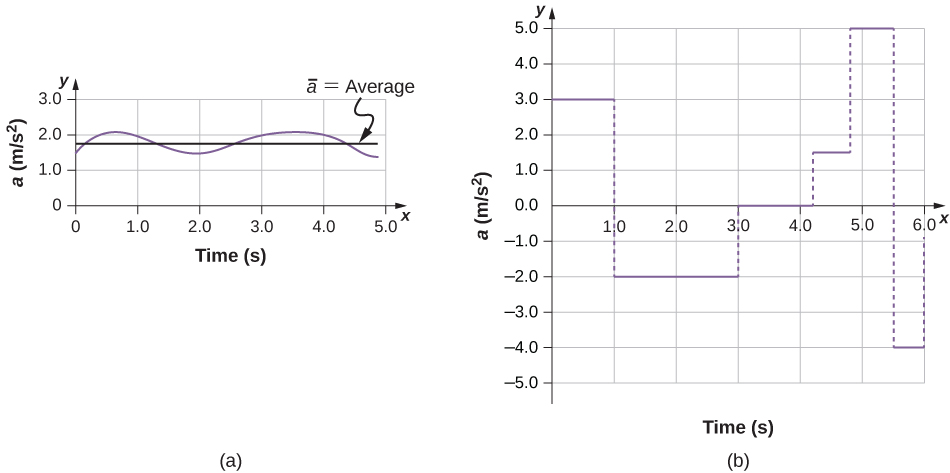
In this table, we see that typical accelerations vary widely with unlike objects and have nothing to practice with object size or how massive it is. Acceleration can as well vary widely with time during the motion of an object. A drag racer has a big dispatch just after its offset, but then it tapers off equally the vehicle reaches a constant velocity. Its boilerplate dispatch can be quite different from its instantaneous acceleration at a item fourth dimension during its motion. Effigy compares graphically boilerplate acceleration with instantaneous dispatch for two very different motions.

Figure three.17 Graphs of instantaneous acceleration versus time for two different one-dimensional motions. (a) Acceleration varies only slightly and is always in the same direction, since it is positive. The boilerplate over the interval is nearly the same equally the dispatch at whatever given time. (b) Dispatch varies greatly, perchance representing a bundle on a mail function conveyor belt that is accelerated forward and backward as information technology bumps forth. It is necessary to consider pocket-sized fourth dimension intervals (such every bit from 0–ane.0 s) with constant or nearly abiding acceleration in such a situation.

Learn about position, velocity, and acceleration graphs. Move the little man back and forth with a mouse and plot his motion. Set up the position, velocity, or dispatch and let the simulation move the homo for you. Visit this link to utilise the moving man simulation.

Summary

• Dispatch is the rate at which velocity changes. Acceleration is a vector; it has both a magnitude and direction. The SI unit for acceleration is meters per 2d squared.
• Acceleration tin be caused by a change in the magnitude or the direction of the velocity, or both.
• Instantaneous acceleration a(t) is a continuous part of time and gives the acceleration at whatever specific time during the motion. It is calculated from the derivative of the velocity office. Instantaneous acceleration is the slope of the velocity-versus-time graph.
• Negative acceleration (sometimes called deceleration) is acceleration in the negative direction in the chosen coordinate system.

Conceptual Questions

Is it possible for speed to exist abiding while acceleration is not zero?

Show Solution

No, in one dimension abiding speed requires nil acceleration.

Is it possible for velocity to exist constant while acceleration is non naught? Explain.

Give an example in which velocity is zero yet dispatch is not.

Bear witness Solution

A brawl is thrown into the air and its velocity is zero at the apex of the throw, just acceleration is non zero.

If a subway railroad train is moving to the left (has a negative velocity) and then comes to a stop, what is the direction of its acceleration? Is the acceleration positive or negative?

Plus and minus signs are used in i-dimensional move to point direction. What is the sign of an acceleration that reduces the magnitude of a negative velocity? Of a positive velocity?

Show Solution

Plus, minus

A cheetah tin can advance from residue to a speed of xxx.0 g/s in vii.00 due south. What is its acceleration?

Show Solution

[latex]a=iv.29{\text{m/s}}^{two}[/latex]

Dr. John Paul Stapp was a U.S. Air Force officer who studied the effects of extreme acceleration on the human body. On December 10, 1954, Stapp rode a rocket sled, accelerating from rest to a top speed of 282 m/s (1015 km/h) in v.00 s and was brought jarringly back to residue in only 1.40 southward. Summate his (a) acceleration in his direction of motion and (b) dispatch opposite to his direction of motion. Express each in multiples of g (9.80 thousand/s²) by taking its ratio to the acceleration of gravity.

Sketch the acceleration-versus-time graph from the following velocity-versus-time graph.

Testify Respond

A commuter backs her car out of her garage with an acceleration of 1.forty chiliad/s². (a) How long does it take her to attain a speed of 2.00 yard/due south? (b) If she so brakes to a stop in 0.800 s, what is her acceleration?

Assume an intercontinental ballistic missile goes from balance to a suborbital speed of 6.fifty km/due south in sixty.0 s (the actual speed and time are classified). What is its average acceleration in meters per 2d and in multiples of g (9.fourscore m/due south²)?

Show Solution

[latex]a=11.1g[/latex]

An airplane, starting from rest, moves down the runway at abiding acceleration for 18 s and then takes off at a speed of 60 m/due south. What is the average acceleration of the aeroplane?

Glossary

average acceleration

the rate of change in velocity; the change in velocity over time

instantaneous acceleration

acceleration at a specific betoken in time

Source: https://pressbooks.online.ucf.edu/osuniversityphysics/chapter/3-3-average-and-instantaneous-acceleration/

Posted by: orozcowarts1946.blogspot.com

Share this post